
At FlyMy.AI, we’re building the fastest Compound AI platform, delivering unparalleled inference speed for all types of neural networks and AI applications. We take pride in our in-depth system implementation, optimizing every component from SIMD kernels to distillation techniques and protocols. This relentless focus on optimization is how we achieved the world’s fastest real-time demo of Diffusion NN , maintaining high image quality without compromising on FPS
For some parts in our system we use Triton, a language and compiler developed by OpenAI, aims to provide better performance than CUDA while using a higher-level language. This allows us to rewrite certain neural network algorithms in Triton, outperforming those in popular Python libraries like PyTorch — while still writing in Python.
In this post, we’ll demonstrate how well-known kernels can be implemented in Triton, showcasing its significant performance improvements. Specifically, we’ll focus on a kernel related to input normalization — Group Normalization.
Normalization techniques are essential in AI because they stabilize and accelerate training by ensuring that inputs to each layer are on a consistent scale, making learning more efficient. In Generative AI (GenAI), these techniques are critical for producing high-quality, realistic outputs. They maintain balance in the data, preventing issues like exploding or vanishing gradients, which can hinder model performance.
Batch Normalization has been the most used algorithm for normalizing layers in deep learning models for quite a while now. It consists of normalizing the channels by using the mean and variance over all batches, however efficiency is diminished if the amount of batches isn’t large
enough (usually at least 32). After the mean and variance of a specific channel are computed, the channel is normalized, then scaled and shifted accordingly..
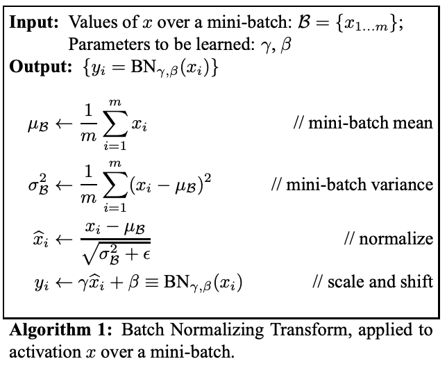
Layer Normalization does the same thing, however over all channels of a specific batch.
Instance Normalization, on the other hand, performs the calculations only over a channel in a batch.
Group Normalization is a mid-term between these methods, in which the calculations are performed over a group of channels of a specific batch; this amount of channels in which the algorithm runs through has to be divisible by the amount of channels in total. The following image describes the relations between each method.

Batch Normalization is a widely used technique known for delivering high-quality results, but Group Normalization (GN) is particularly important in Generative AI and diffusion models. GN enhances the stability and quality of neural networks during training and overcomes the limitations of BatchNorm, which can be problematic in image generation processes.
Specifically:
We’re going to follow using an example of a tensor, whose batch size is 2, with each batch consisting of 4 channels, height 2 and width 2. As such, the example has the shape (N, C, H, W) = (2, 4, 2, 2)
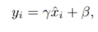
And also, let’s define the following tensors as the weights (also known as gamma) and the bias (also known as beta). These two tensors must have the same length as the amount of channels in the input tensor, as they are applied independently for each channel.
γ = [0.2963, −0.9232, 1.4572, −1.0557]β = [0.0984, 1.2018, −1.0154, 0.0261]
Finally, we define what’s the amount of groups that we’re going to work with. This value needs to be a divisor of the number of channels of the input, and so for this case we must choose between 1, 2 and 4. If we choose 1, we’re pretty much doing the same as layer normalization, and if we
choose 4, it’s going to be the same as instance normalization. To demonstrate the middle-ground that is group normalization, I’m going to choose 2 for this example.
Therefore, the code using the builtin group normalization function from PyTorch should look something like this:
import torcha = torch.tensor( [[[[0.0127, 0.6262], [-0.3884, -0.9077]], [[-0.5615, -0.4755], [-1.2070, 0.2371]], [[1.2504, 0.0138], [-0.5010, 0.3860]], [[-0.2113, 0.8218], [-0.4039, 1.7963]]], [[[0.6527, 1.4151], [-0.3092, -0.4007]], [[0.4586, -1.1754], [-0.3117, -0.9210]], [[-2.5762, 0.6758], [0.4550, 0.1805]], [[-0.3143, -0.8534], [0.8388, 0.7529]]]], device='cuda')groups = 2gamma = torch.tensor([0.2963, -0.9232, 1.4572, -1.0557], device='cuda')beta = torch.tensor([0.0984, 1.2018, -1.0154, 0.0261], device='cuda')res = torch.nn.functional.group_norm(a, groups, gamma, beta, 1e-5)
As such, let’s calculate the value of the element (0, 0, 0, 0) (remembering that the tensor is 0-indexed), by doing the following:


First of all, the implementation of the algorithm will vary depending on how the tensor is configured in memory. This depends on whether or not the format is in channels last or not; for a better understanding check out here. For simplicity reasons, we’re going to work as if the input tensor is
in classic contiguous storage, however the difference to the other one is how we will iterate through the memory.
Loading everything into GPU memory for calculations isn’t efficient, especially when working with large datasets. Some algorithms calculate variance in an online manner, meaning you don’t need the entire dataset at once. This is useful because, for each group where we calculate the mean and variance, dividing it into smaller blocks is faster than processing everything at once.
Join Medium for free to get updates from this writer.
Subscribe
The Welford Combine algorithm is straightforward. It works by storing the running mean and the running squared difference from the mean, similar to the naive method. Here’s how it can be understood:
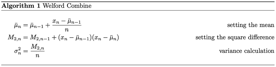
Of course, implementing this linearly would be a bit costly, as you’d have to apply the algorithm having a separate function call for every element, so what we can do is do a bunch at the same time (size being the block size that we’re going to work with) and at the end combine them all by using the function triton.language.reduce. The Welford Combine should then look something like this:
@triton.jitdef welford_combine(mean1, m21, weight1, mean2, m22, weight2): delta = mean2 - mean1 new_weight = weight1 + weight2 w2_over_w = tl.where(new_weight == 0.0, 0.0, weight2/new_weight) return ( mean1 + delta * w2_over_w, m21 + m22 + delta * delta * weight1 * w2_over_w, new_weight, )
For this part, we’re going to use the same example as in the end of section 2, but instead of calling the function from torch, we’re going to create our own group norm function. The initial call is easy to handle, as you only need to work on checking some conditions.
import tritonimport triton.language as tlfrom torch.prims_common import suggest_memory_formatdef group_norm(input, groups, gamma, beta, eps): assert input.is_cuda and gamma.is_cuda and beta.is_cuda N, C, H, W = input.shape assert C % groups == 0 assert gamma.shape == (C,) assert beta.shape == (C,) assert suggest_memory_format(input) != torch.channels_last input = input.contiguous() output = torch.empty_like(input) def grid(meta): return (groups, N) group_norm_kernel[grid](input, gamma, beta, output, N, C, H * W, groups, eps) return output
Our grid function determines how the parallelization of the kernel will work, together with meta-parameters.
Now we get to the harder part of the implementation; our parallelization will occur in two axes: one with the amount of groups and the other with the amount of batches. Let’s look at some constants that will vary depending on the parameters:
@eval('''triton.heuristics({ 'BLOCK_SIZE': lambda kwargs: min(4096, triton.nextpowerof2(kwargs['HW'])),})''')@eval('''triton.heuristics({ 'num_warps': lambda kwargs: max(1, min(16, triton.nextpowerof2(kwargs['HW'] // kwargs['C'] // kwargs['groups']))), 'CG': lambda kwargs: kwargs['C'] // kwargs['groups'], 'GROUP_SIZE': lambda kwargs: kwargs['C'] // kwargs['groups'] * kwargs['HW'],})''')@triton.jitdef groupnorm_kernel( input_ptr, gamma_ptr, beta_ptr, output_ptr, N, C, HW, groups, eps, CG, GROUP_SIZE, BLOCK_SIZE: tl.constexpr,): group = tl.program_id(0) pid_batch = tl.program_id(1) offset = pid_batch * C * HW + group * GROUP_SIZE input_offset = input_ptr + offset output_offset = output_ptr + offset mean = tl.zeros((BLOCK_SIZE,), dtype=tl.float32) m2 = tl.zeros((BLOCK_SIZE,), dtype=tl.float32) weight = tl.zeros((BLOCK_SIZE,), dtype=tl.float32) for off in range(0, GROUP_SIZE, BLOCK_SIZE): r = off + tl.arange(0, BLOCK_SIZE) x = tl.load(input_offset + r, mask=r < GROUP_SIZE).to(tl.float32) m2 = tl.zeros((BLOCK_SIZE,), dtype=tl.float32) weight = (r < GROUP_SIZE).to(tl.float32) mean, m2, weight = welford_combine(mean, m2, weight, x, m2, weight) mean, m2, weight = tl.reduce((mean, m2, weight), 0, welford_combine) var = m2 / weight rstd = 1.0 / tl.sqrt(var + eps) for c in range(0, CG): gamma = tl.load(gamma_ptr + group * CG + c).to(tl.float32) beta = tl.load(beta_ptr + group * CG + c).to(tl.float32) a = rstd * gamma b = beta - a * mean for off in range(0, HW, BLOCK_SIZE): r = off + tl.arange(0, BLOCK_SIZE) x = tl.load(input_offset + c * HW + r, mask=r < HW).to(tl.float32) x = a * x + b tl.store(output_offset + c * HW + r, x, mask=r < HW)
If necessary, an activation function can be fused into the kernel. To prevent further function calls and to already use what’s loaded onto the GPU memory, it is possible to use an activation function right before storing the results. The following example will show how the last three lines of code need to be from the example above when using GELU:
x = a * x + bx = 0.5 * x * (1.0 + tl.tanh(0.7978845608028654 * (x + 0.044715 * x * x * x)))tl.store(output_offset + c * HW + r, x, mask=r < HW)
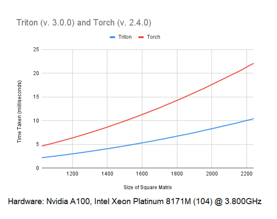
We ran the code using Triton 3.0.0 and Torch 2.4.0. The benchmark consists of a randomly generated tensor with dimensions (1, 32, X, X), where X had the range (64, 96, . . . , 2240). Using 8 groups and having the values of gamma and beta being randomly generated. This ran on a
machine with an Nvidia A100.
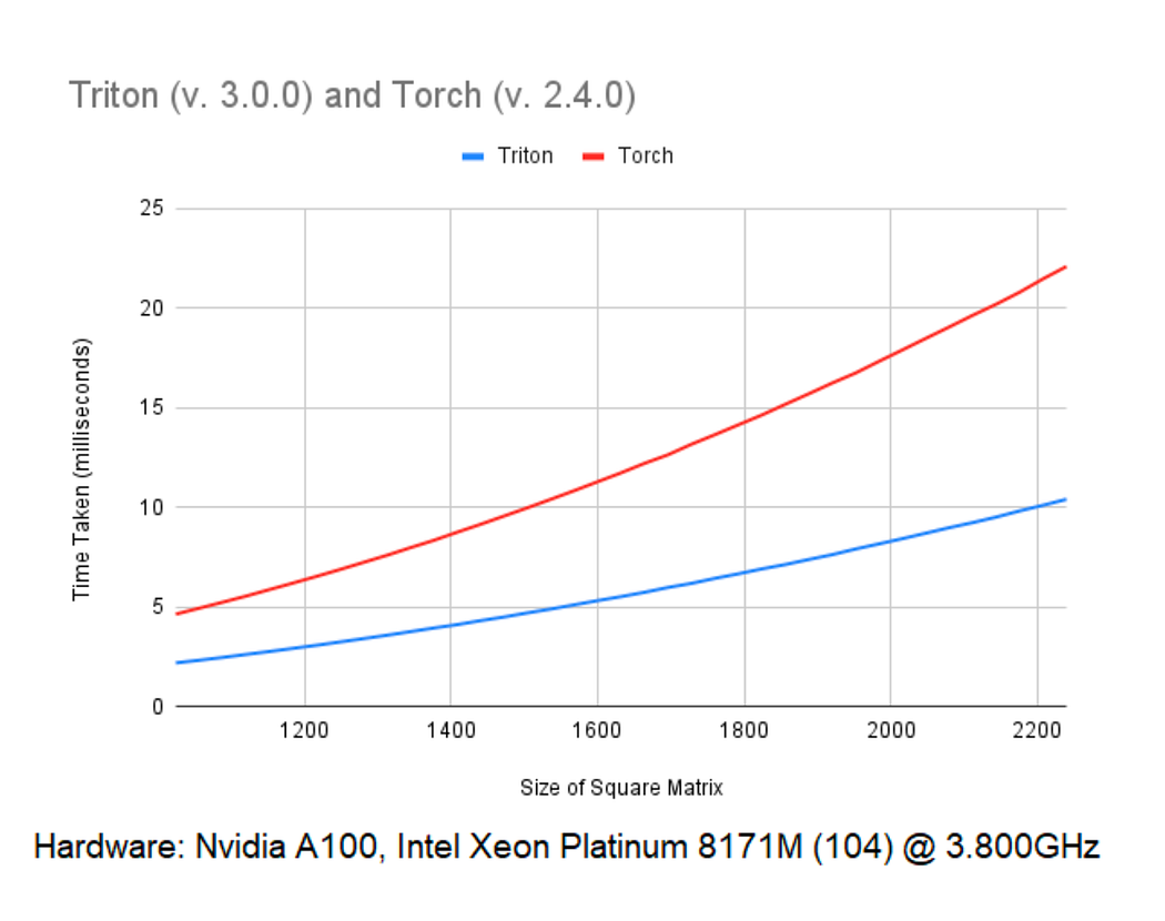
As seen in the graph, Triton kernels work up to 2.5x faster, and difference in performance increases with tensor size. It may seem that implementing kernels in Triton is relatively simple, but this is not the case for some other algorithms. For instance, Triton doesn’t allow access to specific indices during calculations, making it difficult to implement more complex algorithms, such as the Fast Fourier Transform, correctly. As a result, when implementing other kernels, such as Convolution, the performance may be worse than that of the PyTorch library, depending on the input size.